The Journey of a Photon – From Spark to Spectra

The photons used in spectroscopy encounter many components and undergo a variety of processes before registering as a spectrum on the screen. What happens to these photons once they enter an Ocean Insight spectrometer?

1. An Exciting Start

The photons used in spectroscopy may be created through reactions in the sun or stars, or emitted locally from lamp bulbs, LEDs or lasers. Photons can even be excited from everyday materials as fluorescence or Raman scattering. Whatever its origin, each photon is created with a specific wavelength, which it will carry throughout its lifetime (from mere nanoseconds to billions of years).

 

2. A Bumpy Road to the Slit

As photons travel through space, they may be reflected, transmitted, scattered or absorbed by the materials they encounter. By looking at the resulting light as compared to the initial amount of light, it is possible to learn about the properties of the material or sample encountered. This is because the probability of a photon interacting with a material in a certain way varies with that material’s chemical and physical structure, and with the wavelength of the photon itself. Each interaction with a material will filter, redirect or simply eliminate photons of various wavelengths.

 

3. A Guided Path 

Fiber optic cables are a convenient method to safely route light from one point to another. Multimode fibers guide light through total internal reflection, acting as a light pipe to redirect light from one location to another without interference from ambient light. A fiber can even “bend” light around corners, and greatly simplifies the process of routing light to a spectrometer.

Most Ocean Insight fibers use an SMA 905 connector at their tip to connect the spectrometer, providing a snug, alignment-free coupling between the fiber’s end and the entrance point into the spectrometer: the slit.

 

4. Single File, Please! 

The slit is a very narrow aperture through which a stream of well-directed photons traveling in a consistent direction can flow. A typical slit is only 1 mm tall, and anywhere from 5 μm to 200 μm wide. Most slits are rectangular, but some may be oval for improved optical performance. The wider the slit, the more photons can get through (higher throughput), but at the cost of reduced optical resolution (higher FWHM, which means some peaks may appear wider than they are).

 

5. Collimation 

The photons entering through the slit are still diverging in space (the beam expands after passing through the slit), so their first port of call is a collimating mirror. This has a focusing effect to help the photons travel parallel to one another, so they won’t scatter in unwanted directions.

 

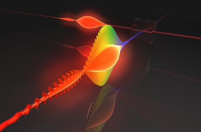
6. Diffraction 

The collimating mirror simultaneously reflects the photons to a reflective diffraction grating, which splits photons out by wavelength. “Blue” photons (around 450 nm) are reflected at one angle, while “red” photons (around 700 nm) are reflected at a larger angle. This is the most important step in separating the collected light by wavelength, allowing each wavelength to be measured discretely.

 

7. Focus Carefully Now 

After leaving the diffraction grating, the newly dispersed light is sent to a focusing mirror, which reflects light of each wavelength onto the detector while focusing it slightly. The detector is a linear array of CCD pixels – similar to a digital camera, but in a 1-dimensional line instead of a 2D rectangle. Each pixel collects photons from a very narrow range of wavelengths.

 

8. Expect Trade-offs 

Spectrometer range and resolution are a function of the configuration. A narrower spectral range generally allows higher resolution for applications such as laser characterization, while a wider range can often mean lower resolution, which is acceptable for general chemical studies like protein absorbance. However, range and resolution trade-offs can be minimized with the use of a larger-bench spectrometer and extended-range diffraction gratings.

 

9. Charge! 

Each pixel of the detector acts as a well that collects photons of a specific wavelength range. The well starts each integration period “full” of voltaic charge. Each time a photon strikes the well, a bit of that charge is depleted. The longer the integration time, the more photons can be collected at each pixel; however, once the charge is fully depleted, that pixel is “saturated” and no new signal can be collected. In effect, each photon is consumed as it strikes the detector and its energy is released; we will not see it again.

 

10. Enter the Matrix 

At the end of each integration period, the charge level is read from all pixels on the detector. This read-out is passed into an ADC (analog-to-digital converter), which converts each pixel’s voltage into a specific number of “counts.” From this point onward, we’ll be following the digital “intensity counts” (or spectrum) as it moves through the electronics.

 

11. Dynamic Range 

When converting the analog voltage of each pixel into a discrete quantity, the resolution of the ADC plays a part in determining the dynamic range of the spectrum. A 12-bit ADC can only represent values from 0 to 4095 (212), so the greatest range between the highest peak and the baseline is 4096 counts. In contrast, a 16-bit ADC can show discrete wavelength intensities from 0 to 65,535 (216), and an 18-bit ADC can provide even more.

 

12-13. From Electrical Charge to PC 

The spectrum is copied over USB from the spectrometer’s microcontroller to the host PC over USB. Different USB versions transmit data at different speeds, which can affect the scan rate (number of spectra that can be read per second). Also, there are other communication buses avail¬able besides USB, including RS-232, Bluetooth, Ethernet and Wi-Fi, each with its own advantages and pitfalls.

 

14. The Final Drive 

Reading a spectrum over USB doesn’t have to be complicated for the user, but there are a lot of things that have to be done correctly. Fortu¬nately, most of the very low-level USB functions have already been automated by low-level USB device drivers that come for free with modern computer operating systems. Also, at Ocean Insight we have automated most of the higher-level spectrometer control functions using application drivers. With a few lines of code, users will be able to read and process spectra easily using their preferred mix of drivers.

 

15. How Low Can You Go? 

There are several good USB drivers for Windows, including Cypress ezUSB and Microsoft’s own WinUSB (best for 64 bit). Both Linux and MacOS use the open-source libusb. Ocean Insight high-level drivers “wrap” or “call into” these third-party drivers so that you don’t have to learn their sometimes arcane conventions.

 

16. Application Drivers 

Ocean Insight application drivers and software development kits provide high-level function calls like getSpectrum() and setIntegrationTime() to control your spectrometer and retrieve data. 

Drivers can be used from a variety of programming languages and platforms to quickly compile custom spectroscopy applications and GUIs. C, C++, C#, LabVIEW, and many other targets are supported.

 

17. Post-Processing Spectra 

Various techniques are available to process your spectral data: 
●  Electrical Dark Correction (EDC): Subtract averaged “optically masked dark pixels” to correct for readout noise and thermal drift. 
●  Non-Linearity Correction (NLC): Apply a factory-calibrated 7th-order polynomial to correct for pixel response as the detector approaches saturation. 
●  Boxcar Averaging: Smooth high-frequency noise by averaging each pixel with its neighbors. 
●  Scan Averaging: Improve signal-to-noise ratio (SNR) by averaging multiple spectra.

 

18. Journey’s End 

This concludes our photon’s journey. From its creation, to its travels within the spectrometer, to its arrival at the detector pixel cell, the photon navigates an inevitable path. 

As each photon’s “fate” is recorded and digitized into data, additional stops along the way lead us to graphable spectra in a format we can understand. With more sophisticated spectral processing using machine learning, we can turn data into insights – the answers you seek.

 

Article Source:  https://www.oceaninsight.com/globalassets/catalog-blocks-and-images/app-notes/journey-of-a-photon_technote.pdf